Mortis

Mortis · Python

The same amount,
arranged differently.

Imaging mass spectrometry tells you where a metabolite is, then most analyses throw that away and ask only how much. MORTIS tests both, at the patient level, where the statistics are actually valid.

pip install mortis-spatial Quickstart
acquiring · 25 µm raster

The flaw this package exists to fix

A tissue section has 30,000 pixels and one patient.

Test those pixels as independent replicates and you inflate your sample size by four orders of magnitude. The p-values that come out are not small because the biology is strong. They are small because n is wrong.

Here is what that costs, measured. Six simulated patients, three per arm, 500 pixels each, 200 metabolites, and no group difference at all, only the ordinary variation between patients:

Pixel-level test · n = 1,500 per arm 0/200

metabolites called significant at FDR < 0.05, on data containing nothing to find. Roughly 92% of the findings were manufactured by the method.

Patient-level test · n = 3 per arm 0/200

significant. The correct answer, from the same data, by counting patients instead of pixels.

This is not a subtle statistical preference. It is the difference between a result and an artefact, and it is documented for imaging mass spectrometry specifically, a published pixel-level t-test reporting P = 9.6 × 10⁻⁷ where the correct patient-level test gives P = 0.78.

So pseudobulk() comes first, and the pixel-level function still available for genuine within-section comparisons raises a warning that names the risk.

What imaging can see that bulk cannot

Two sections. Identical total signal.

Abundance testing asks whether there is more of something, which is the question bulk metabolomics already answers. Run it on imaging data and you have paid for spatial resolution to discard it.

A metabolite can sit at exactly the same abundance in two patients and be arranged completely differently: diffuse and even in one, pooled into sharp foci in the other. Lactate spread through a section and lactate concentrated in hypoxic cores are not the same biology, and no abundance test can tell them apart.

Step one

Measure how much.

pseudobulk() collapses every pixel in a section to one profile per patient. Twelve sections, twelve numbers per metabolite, the unit the statistics are actually valid at.

Spermidine comes back identical in both arms. Cliff's δ = 0.00. A bulk experiment would stop here and report nothing.

Step two

Then measure how it sits.

spatial_organization() collapses the same sections to arrangement instead. Moran's I, normalised entropy, Gi* hotspot fraction, Gini. One number per section per metabolite, scale-free so a big biopsy cannot outscore a small one.

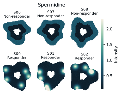
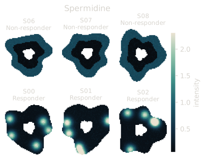
Every responder concentrates spermidine into a focus. Every non-responder spreads it. δ = 1.00, FDR = 0.002.

Step three

Ask which axis moved.

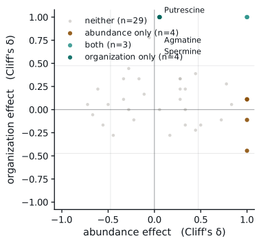
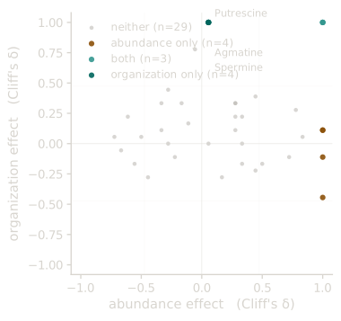
compare_abundance_and_organization() places every metabolite on both and labels it. Four polyamines land at abundance δ = 0, organization δ = 1.0.

Same amount. Different arrangement. Only imaging can see this, and only if you look for it.

Spermidine across twelve sections: responders focal, non-responders diffuse.
Abundance effect against organization effect; four polyamines at zero abundance and maximal organization effect.

And the honest part

This needs six sections per group. Measured, not assumed: on a benchmark with three planted organization-only differences among thirty metabolites, effect size alone over-called at every cohort size, while effect size plus FDR gave exactly three true and zero false positives from n = 6 upward, and nothing at all below it. A Mann-Whitney comparison of five against five bottoms out at p = 0.0079, which cannot survive multiple-testing correction. Below six, an empty result is the correct answer.

End to end

Instrument export to submitted figure.

Eleven stages on one AnnData object. Every stochastic step takes a seed; every seeded step gives the same answer on a different machine.

Quickstart

The whole cohort analysis

import mortis as mt

# Load, clean, normalise
adatas       = mt.load_from_folder("./sections")
clean, stats = mt.filter_background(adatas, cutoff=1.5)
adata        = mt.preprocess(mt.merge_samples(clean))

# Collapse pixels to patients, never test pixels across patients
pb  = mt.pseudobulk(adata, sample_key="patient")
org = mt.spatial_organization(adata, sample_key="section")

# Test both axes at the patient level
ab   = mt.differential_abundance(pb,  "response", "R", "NR")
do   = mt.differential_spatial_organization(org, "response", "R", "NR")
both = mt.compare_abundance_and_organization(ab, do)

# Identifiers and pathways, in one call
ids, paths = mt.annotate_pathways(adata, ab)

# Figures, vector PDF, text stays editable
mt.set_publication_style(latex=True)
fig = mt.plot_abundance_vs_organization(both)
mt.save_figure(fig, "figures/fig3", provenance={"cohort": "vedo", "seed": 0})
Command by command

What each call gives you back.

The quickstart above is the whole analysis in twenty lines. This is the same run opened up, what goes in, what comes out, and what you do with it next.

For the reviewer

Prove it reproduces, without sending the data.

"Available on reasonable request" verifies nothing. A reviewer who doubts a result can take it on trust, ask for data the ethics approval forbids sharing, or reimplement your methods paragraph. None of those is checking.

export_manifest() writes a sealed JSON recording the environment, every step and its seeds, and a checksum of the inputs and of every result table. verify_manifest() re-runs the comparison and names precisely what diverged.

Checksums are one-way. Nothing in the file can be turned back into an intensity, so it is safe to attach to a submission for a cohort that can never leave the institution, which is the situation clinical imaging data is always in.

# after the analysis
mt.export_manifest("manifest.json", adata=pb,
                   results={"abundance": ab, "organization": do},
                   analysis="vedolizumab week 14")

# anyone re-running it, months later
report = mt.verify_manifest("manifest.json", adata=pb, results=...)

Output

Figures you can hand to a co-author.

PDF text stays text, embedded TrueType with a character map, so a collaborator can retype a label in Illustrator and a reviewer can search the file. Only dense scatter interiors are rasterised; axes and labels never are.

Every figure carries its analysis parameters and a hash in the PDF metadata, so pdfinfo figure.pdf identifies the run that made it months later.

Does it work on real data

A public study, start to finish, using nothing else.

Everything above is a claim about the package. This is the package run against openly available data by a script anyone can execute, no simulation, no private cohort, no other tool in the pipeline.

The study is 2026_Frank_solanum_recal on METASPACE: MALDI imaging of grafted Solanum stems. Ion images are downloaded, reconstructed into pixel matrices, and taken through cleaning, pseudobulk, sample-level testing, spatial organization, chemical classification and a sealed manifest.

The controls

A method that finds everything is worth nothing.

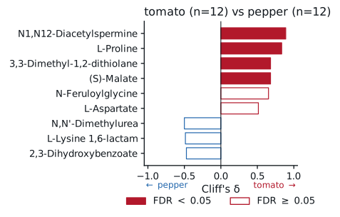
Positive control, tomato versus pepper tissue. Two different plants. A working method has to find something, and it does: four ions separate them at FDR < 0.05 across 24 sections, led by N1,N12-Diacetylspermine (δ = +0.89) and L-Proline (δ = +0.83).

Underpowered control, position within homo-grafts. Holding species constant leaves only three sections per arm, below the six-per-arm floor MORTIS documents. It returns nothing, which is the correct answer rather than a disappointing one.

A trap the script refuses. "Top versus bottom" looks like the obvious contrast and is not: on a tomato-pepper graft the section above the junction is tomato and the one below is pepper, so position is a species contrast wearing a different label. Run naively across all grafts it returns nothing at all.

Two further things worth reporting rather than hiding: five sections carry condition metadata that contradicts their own name, so grouping follows the name; and zero ions differ on spatial organization here, an honest null on this tissue.

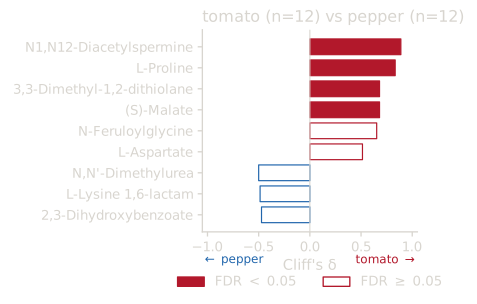
Cliff's delta for the strongest ions separating tomato from pepper tissue.
Tomato versus pepper across 24 public sections and 250,514 pixels. Solid bars clear FDR < 0.05. Every figure and table on this page came out of validation/run_validation.py, cached so a rerun costs no downloads and reproduces exactly.

Reproduce it

# fetches the public study, runs everything, writes a sealed manifest
python validation/run_validation.py --sections 12 --ions 40

# then check your run against ours
mt.verify_manifest("validation/results/manifest.json", adata=pb, results=...)

Reference

Every function, generated from the package.

Pulled from the installed module at build time, so this cannot drift from the code. Search, or filter by stage.

Why you can trust the output

Correctness is a claim you have to be able to check.

Every number here is measured on this machine and pinned by a test that fails on the code as it stood before the fix.

Spatial statistics stream over metabolite tiles, so a cohort that used to need 4.3 GB of working memory now needs 0.99 GB and runs twice as fast, with bit-identical checksums. Sparse and disk-backed matrices give the same answers as dense ones, and tile size is a memory dial that never changes a result.